
03-1. k-최근접 이웃 회귀
k-최근접 이웃 회귀
- 지도 학습 알고리즘은 크게 분류와 회귀로 나뉨
- 분류는 말 그대로 샘플을 몇 개의 클래스 중 하나로 분류하는 문제
- 회귀는 클래스 중 하나로 분류하는 것이 아니라 임의의 어떤 숫자를 예측하는 문제
Why? - k-최근접 이웃 알고리즘은 어떻게 숫자를 예측할 수 있는가?
- 먼저 예측하려는 샘플에 가장 가까운 샘플 k개를 선택
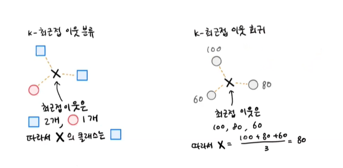
- 이 샘플들의 클래스를 확인하여 다수 클래스를 새로운 샘플의 클래스로 예측
ex) k=3(샘플이 3개)이라 가정하면 사각형이 2개로 다수이기에 새로운 샘플의 x의 클래스는 사각형이 됨
k-최근접 이웃 회귀도 마찬가지다

- 분류와 똑같이 예측하려는 샘플에 가장 가까운 샘플 k개를 선택함
- but 회귀 = 이웃한 샘플의 타깃 어떤 클래스 x, 임의의 수치임
- 이웃 샘플 수치를 사용 -> 새로운 샘플 x를 찾는 방법은? -> 이 수치들의 평균을 구하면 됨
- 이웃한 샘플의 타깃값 -> 100, 80,60임 -> 이를 평균하면 x의 타깃값은 80
데이터 준비
코드1 - 훈련 데이터 준비
import numpy as np
perch_length = np.array([8.4, 13.7, 15.0, 16.2, 17.4, 18.0, 18.7, 19.0, 19.6, 20.0, 21.0,
       21.0, 21.0, 21.3, 22.0, 22.0, 22.0, 22.0, 22.0, 22.5, 22.5, 22.7,
       23.0, 23.5, 24.0, 24.0, 24.6, 25.0, 25.6, 26.5, 27.3, 27.5, 27.5,
       27.5, 28.0, 28.7, 30.0, 32.8, 34.5, 35.0, 36.5, 36.0, 37.0, 37.0,
       39.0, 39.0, 39.0, 40.0, 40.0, 40.0, 40.0, 42.0, 43.0, 43.0, 43.5,
       44.0])
perch_weight = np.array([5.9, 32.0, 40.0, 51.5, 70.0, 100.0, 78.0, 80.0, 85.0, 85.0, 110.0,
       115.0, 125.0, 130.0, 120.0, 120.0, 130.0, 135.0, 110.0, 130.0,
       150.0, 145.0, 150.0, 170.0, 225.0, 145.0, 188.0, 180.0, 197.0,
       218.0, 300.0, 260.0, 265.0, 250.0, 250.0, 300.0, 320.0, 514.0,
       556.0, 840.0, 685.0, 700.0, 700.0, 690.0, 900.0, 650.0, 820.0,
       850.0, 900.0, 1015.0, 820.0, 1100.0, 1000.0, 1100.0, 1000.0,
       1000.0])
코드2 - 데이터가 어떤 형태를 띠고 있는지 산점도 그리기
import matplotlib.pyplot as plt
plt.scatter(perch_length, perch_weight)
plt.xlabel('length')
plt.ylabel('weight')
plt.show()
코드3 - 훈련 세트와 데이터 세트로 나누기
from sklearn.model_selection import train_test_split
train_input, test_input, train_target, test_target = train_test_split(perch_length, perch_weight, random_state=42)
코드4 - 넘파이 크키를 바꿀 수 있는 reshape() 메서드
test_array = np.array([1,2,3,4])
print(test_array.shape)
코드5 - (2,2) 크기로 바꾸기
test_array = test_array.reshape(2,2)
print(test_array.shape)
코드6 - train_input, test_input 2차원 배열로 바꾸기
train_input = train_input.reshape(-1,1)
test_input = test_input.reshape(-1,1)
print(train_input.shape, test_input.shape)
결정계수(R2)
- 사이킷런에서 k-최근접 이웃 회귀 알고리즘을 구현한 클래스 -> KNeighborsRegressor
- 이 클래스의 사용법은 KNeighborsRegressor와 매우 비슷함
- 객체를 생성하고 fit() 매소드로 회귀 모델 훈련!!
from sklearn.neighbors import KNeighborsRegressor
knr = KNeighborsRegressor()
knr.fit(train_input, train_target)
코드7 - 테스트 점수 확인
print(knr.score(test_input, test_target))
- 분류의 경우 테스트 세트에 있는 샘플을 정확하게 분류한 개수의 비율
- 정확도라고 불리며, 정답을 맞힌 개수의 비율
- 회귀에서 정확한 숫자를 맞힌다는 것은 거의 불가능
- why? -> 예측하는 값이나 타깃 모두 임의의 수치여서

- 회귀의 경우 조금 다른 값으로 평가함 -> 이 점수를 결정계수라고 부르거나 또는 R2라고도 부름
- 이 값을 계산하는 방법은 다음과 같음
- 각 샘플의 타깃과 예측한 값의 차이를 제곱하여 더함
- 타깃과 타깃 평균의 차이를 제곱하여 더한 값으로 나눔
- 만약 타깃의 평균 정도를 예측 -> R2는 0에 가까워짐
- 예측이 타깃에 아주 가까워지면 -> 1에 가까운 값이 됨
코드8 - 예측의 절댓값 오차를 평균하여 반환
from sklearn.metrics import mean_absolute_error

# 테스트 세트에 대한 예측을 만든다
test_prediction = knr.predict(test_input)

#테스트 세트에 대한 평균 절댓값 오차를 계산함
mae = mean_absolute_error(test_target, test_prediction)
print(mae) -> 19.157142857142862
과대적합 vs 과소적합
코드9 - 훈련한 모델을 이용한 훈련세트의 R2점수 확인
print(knr.score(train_input, train_target))
- 만약 훈련세트에서 점수가 좋았는데 테스트 세트에서 점수가 bad -> 모델이 훈련세트에 과대적합됨
- 훈련 세트보다 테스트 세트의 점수가 높거나 두 점수가 모두 너무 낮은 경우 -> 훈련세트에 과소적합됨
코드10 - n_neighbors 속성값 바꾸기
#이웃의 개수를 3으로 설정함
knr.n_neighbors = 3

# 모델을 다시 훈련함
knr.fit(train_input, train_target)
print(knr.score(train_input, train_target))
코드11 - 테스트 세트 점수 확인
print(knr.score(test_input, test_target))
- 테스트 세트의 점수는 훈련 세트보다 낮아짐 -> 과소적합 문제 해결
전체코드
"""# k-최근접 이웃 회귀"""

"""# 데이터 준비 """

import numpy as np
perch_length = np.array([8.4, 13.7, 15.0, 16.2, 17.4, 18.0, 18.7, 19.0, 19.6, 20.0, 21.0,
       21.0, 21.0, 21.3, 22.0, 22.0, 22.0, 22.0, 22.0, 22.5, 22.5, 22.7,
       23.0, 23.5, 24.0, 24.0, 24.6, 25.0, 25.6, 26.5, 27.3, 27.5, 27.5,
       27.5, 28.0, 28.7, 30.0, 32.8, 34.5, 35.0, 36.5, 36.0, 37.0, 37.0,
       39.0, 39.0, 39.0, 40.0, 40.0, 40.0, 40.0, 42.0, 43.0, 43.0, 43.5,
       44.0])
perch_weight = np.array([5.9, 32.0, 40.0, 51.5, 70.0, 100.0, 78.0, 80.0, 85.0, 85.0, 110.0,
       115.0, 125.0, 130.0, 120.0, 120.0, 130.0, 135.0, 110.0, 130.0,
       150.0, 145.0, 150.0, 170.0, 225.0, 145.0, 188.0, 180.0, 197.0,
       218.0, 300.0, 260.0, 265.0, 250.0, 250.0, 300.0, 320.0, 514.0,
       556.0, 840.0, 685.0, 700.0, 700.0, 690.0, 900.0, 650.0, 820.0,
       850.0, 900.0, 1015.0, 820.0, 1100.0, 1000.0, 1100.0, 1000.0,
       1000.0])

import matplotlib.pyplot as plt
plt.scatter(perch_length, perch_weight)
plt.xlabel('length')
plt.ylabel('weight')
plt.show()

from sklearn.model_selection import train_test_split
train_input, test_input, train_target, test_target = train_test_split(perch_length, perch_weight, random_state=42)

test_array = np.array([1,2,3,4])
print(test_array.shape)

test_array = test_array.reshape(2,2)
print(test_array.shape)

# 아래 코드의 주석을 제거하고 실행함녀 에러가 발생함
# test_array = test_array.reshape(2,3)

train_input = train_input.reshape(-1,1)
test_input = test_input.reshape(-1,1)
print(train_input.shape, test_input.shape)

from sklearn.neighbors import KNeighborsRegressor

knr = KNeighborsRegressor()

# k-최근접 이웃 회귀 모델을 훈련합니다

knr.fit(train_input, train_target)

print(knr.score(test_input, test_target))

from sklearn.metrics import mean_absolute_error

# 테스트 세트에 대한 예측을 만듬
test_prediction = knr.predict(test_input)

# 테스트 세트에 대한 평균 절댓값 오차를 계산함
mae = mean_absolute_error(test_target, test_prediction)
print(mae)

# 과대적합 vs 과소적합"""

print(knr.score(train_input, train_target))

# 이웃의 개수를 3으로 설정합니다
knr.n_neighbors = 3

# 모델을 다시 훈련합니다
knr.fit(train_input, train_target)
print(knr.score(train_input, train_target))

print(knr.score(test_input, test_target))'공부 기록일지' 카테고리의 다른 글
| 유성이의 공부일지(17-2) - 혼자공부하는 머신러닝 + 딥러닝 2장 (0) | 2024.09.21 |
|---|---|
| 유성이의 공부일지(17-1) - 혼자공부하는 머신러닝 + 딥러닝 2장 (1) | 2024.09.07 |
| 유성이의 공부일지(16) - 혼자공부하는 머신러닝 + 딥러닝 1장 (3) | 2024.08.27 |
| 유성이의 공부일지(15) - 혼자공부하는 컴퓨터 구조 + 운영체제 15장 (0) | 2024.07.16 |
| 유성이의 공부일지(14) - 혼자공부하는 컴퓨터 구조 + 운영체제 14장 (0) | 2024.07.15 |